


Research
Global hydrology is concerned with the role of the terrestrial hydrological cycle in System Earth. In particular it focuses on the role of climate variability on global hydrology and the modelling of global water scarcity and groundwater depletion. To this purpose we have built a next-generation global hydrological model PCR-GLOBWB. The model has been used in various global or continental change analyses, such as the assessment of global nutrient dynamics, methane emissions, global water stress assessment, global flood risk analysis and global seasonal streamflow forecasting.
Our global hydrological research encompasses the following focus areas:
Global Water Scarcity and groundwater depletion
Global population and economic growth and the expansion of irrigated areas lead to an exponential increase in human water use since the 1960. Climate change on the other hand is expected to increase the probability and severity of droughts in already drought-prone areas of the world. The result is an increasing gap between water availability and human water demand, leading to water scarcity or water stress. We have developed the global hydrological model PCR-GLOBWB to model water availability. At the same time we have developed scripts to estimate human water demand from socio-economic data (land cover, GDP, population density, electricity use etc.). PCR-GLOBWB 1.0 and the water demand scripts PCR-GDEM operate at 0.5o globally, are coded in PCRaster and available for download. We have recently developed PCR-GLOBWB 2.0 that operates at 6 minutes globally and is coded in PCRaster-Python.
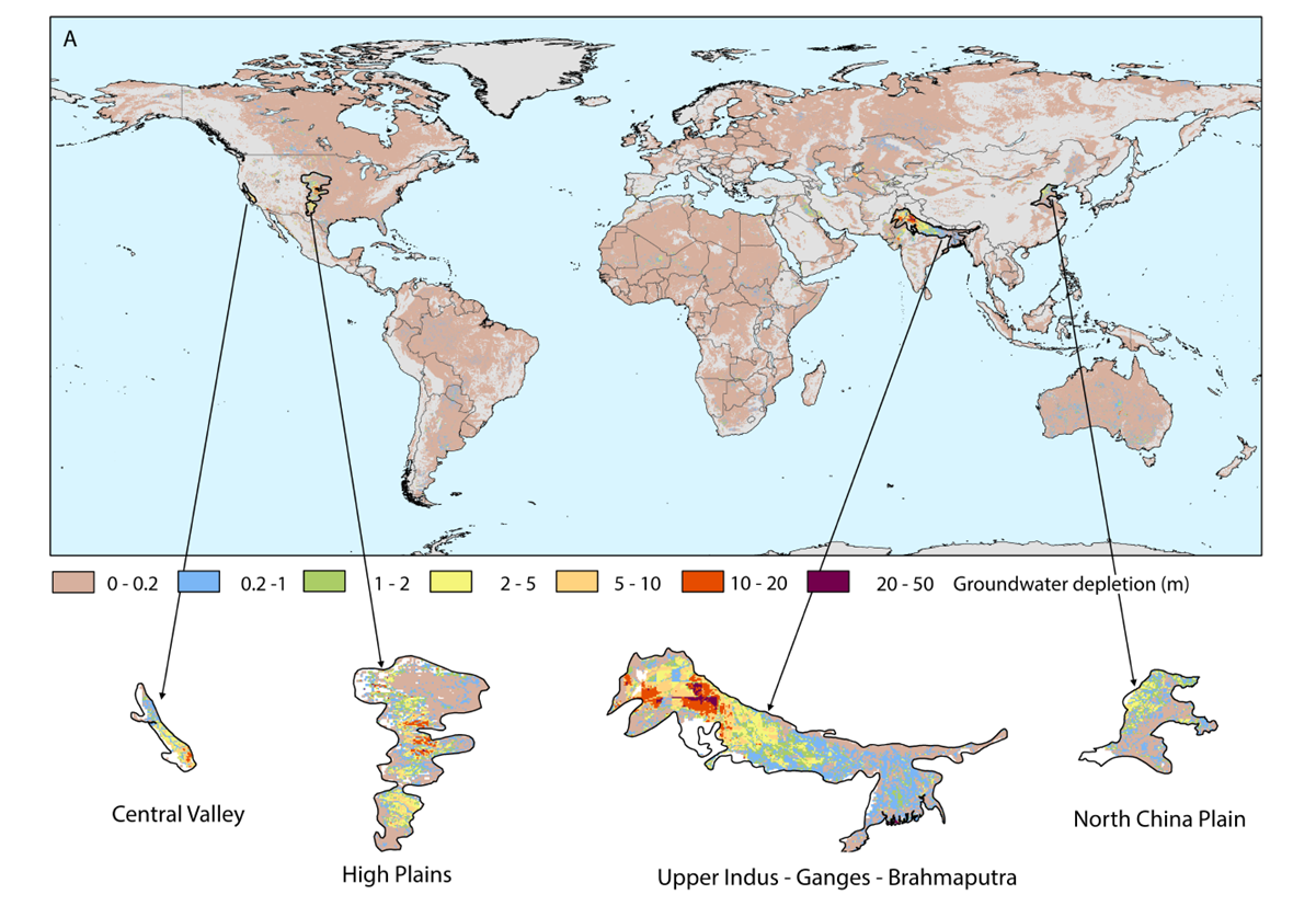
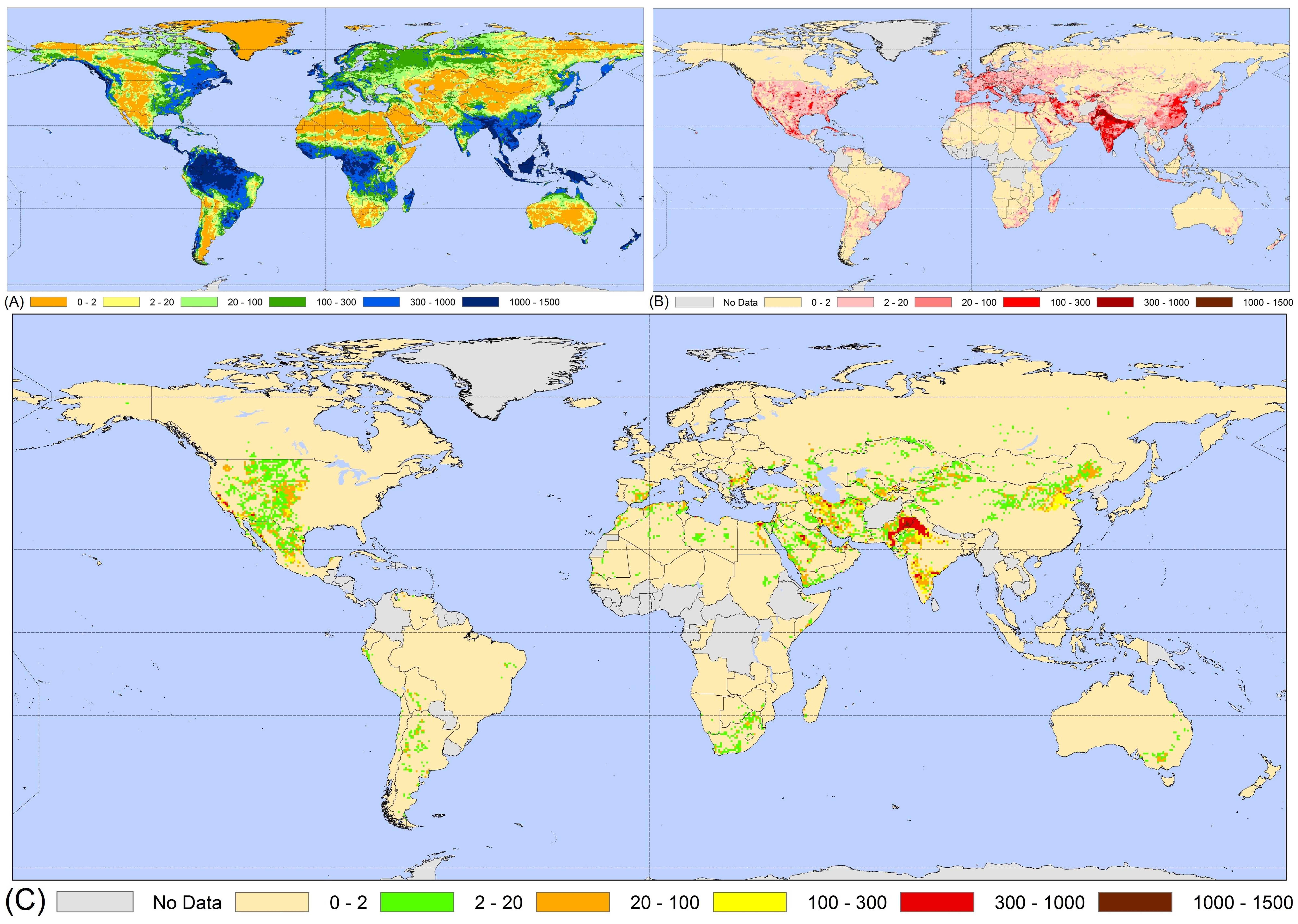 a) Simulated yearly average groundwater recharge by PCR-GLOBWB (1960-2000), b) total groundwater abstraction for the year 2000 and c) groundwater depletion (all figures in 10-3 km3 a-1). d) movie showing development of groundwater depletion 1960-2000 (Source: Wada, et al, 2010, Global depletion of groundwater resources. Geophysical Research Letters L20402).
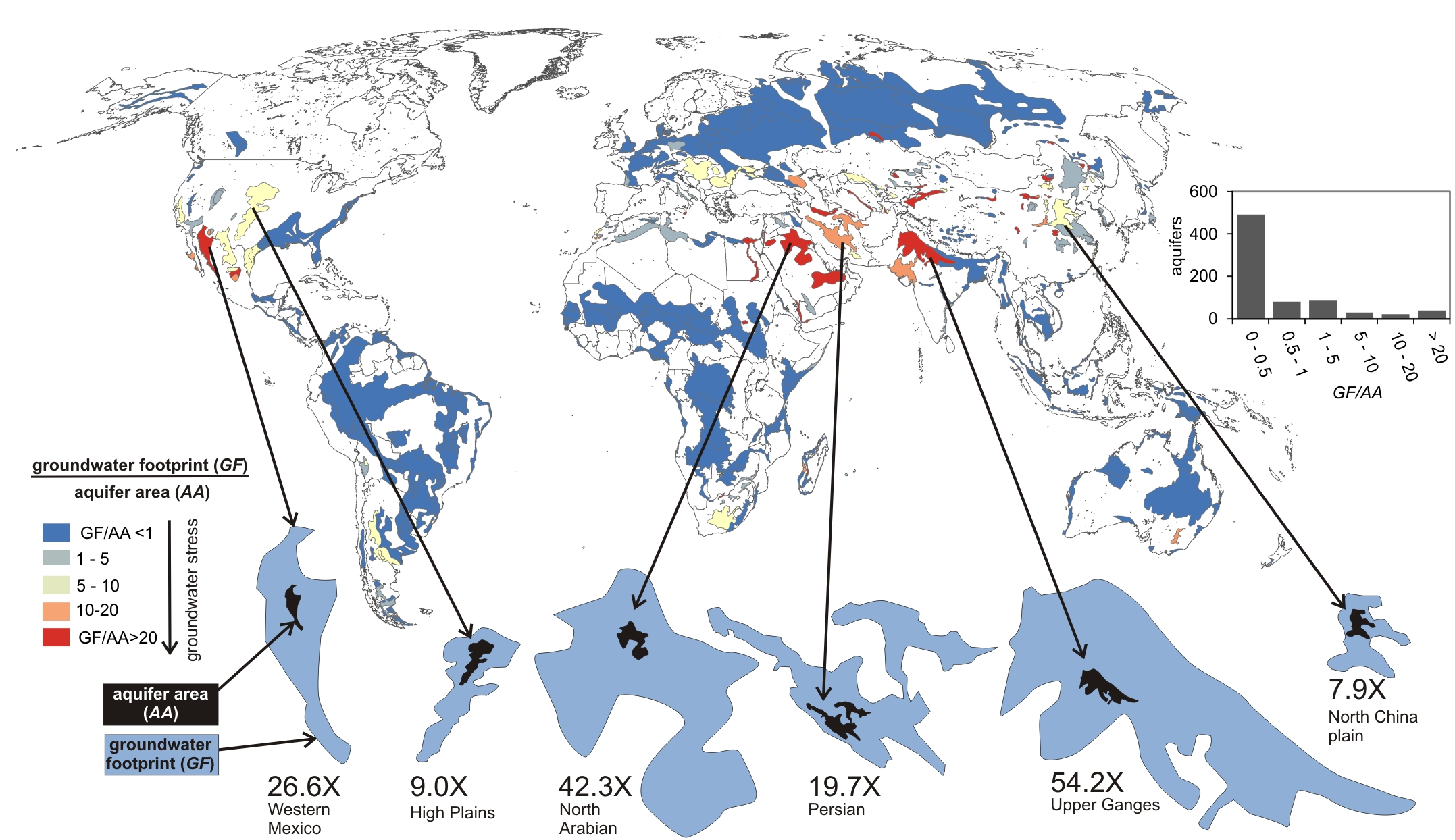
The Groundwater footprint: The dark-blue areas have a groundwater footprint of less than 1; groundwater extraction is sustainable here in the long term as well. However, the red areas in Northern America and Asia have a much larger groundwater footprint. The footprint of the Upper Ganges is actually 54 times larger. The area would have to be 54 times larger to capture the precipitation needed to sustain current groundwater extraction. Groundwater in areas with a large groundwater footprint is severely depleted. The bar chart shows that the groundwater footprint is less than 1 for most areas (80%). The groundwater is being used sustainably here (Source: Gleeson et al., Water balance of global aquifers revealed by groundwater footprint. Nature 488 197–200).
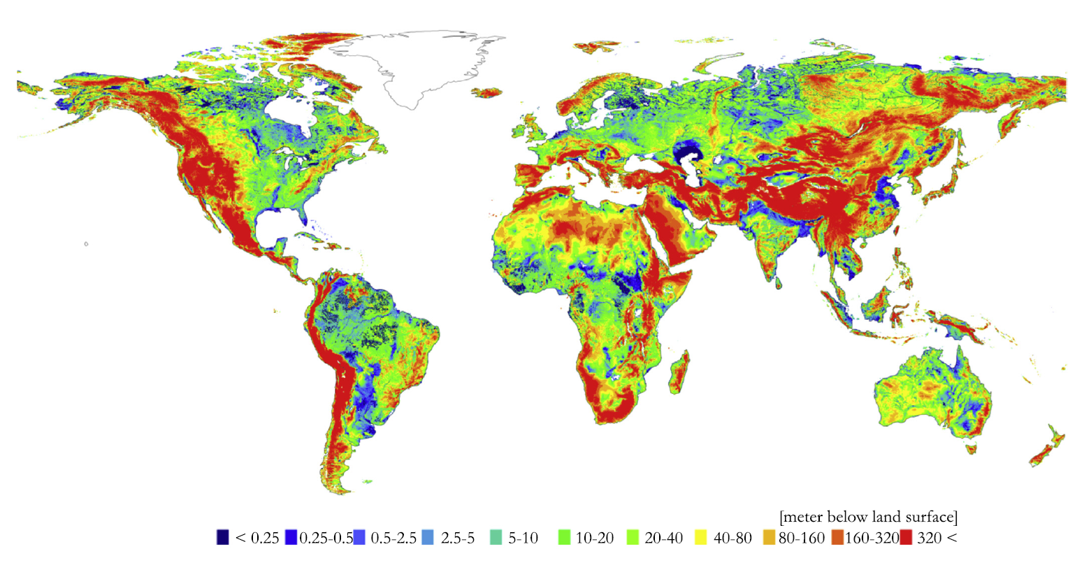
Our recent research computes groundwater depletion with a two-layer transient groundwater model. This enables not only the calculation of depletion rates but also the effects on groundwater levlels and heads. This is neccessary: a) estimate the effects of groundwater withdrawal on other sectors, including wetlands aquatic ecosystems; b) if estimates of volume of groundwater are available, estimate the time to depletion. Our current global groundwater model is at 5 arc-minutes (~10 km) and can be fully coupled ith PCR-GLOBWB 2. We also have first results of a two-layer global groundwater model at 30 arc-seconds (~ 1km).
Groundwater heads (top) and groundwater depletion (bottom) calculated with a global-scale two-layer 5 arc-minutes transient groundwater model based on MODFLOW (Source: De Graaf et al. 207. A global-scale two-layer transient groundwater model: Development and application to groundwater depletion. Advances in Water Resources 102, 53-67)
First results (groundwater heads) of a preliminary 2-layer very high-resolution steady-state groundwater model using MODFLOW 6; model with 428 Million active cells (30 arc-second resolution and 2 vertical layers); decomposed into 1024 subdomains with individual submodels using between 2 and 612 cores; 3 minutes computation time (with favourable starting heads) on the Cartesius Cluster of SurfSARA (Work of Jarno Verkaik, PhD)
Example publications
- Wada, Y., L. P.H. van Beek, C. M. van Kempen, J. W.T.M. Reckman, S. Vasak, and M. F.P. Bierkens, 2010. Global depletion of groundwater resources. Geophysical Research Letters L20402.
- Van Beek, L.P.H., Y. Wada and Bierkens, M.F.P. 2011. Global monthly water stress: 1. Water balance and water availability, Water Resources Research 47, W07517.
- Wada, Y., L.P.H. van Beek, D. Viviroli, H.H. Dürr, R. Weingartner, and M.F.P. Bierkens, 2011. Global monthly water stress: 2. Water demand and severity of water stress, Water Resources Research 47, W07518.
- Wada, Y., L.P.H. van Beek, F.C. Sperna Weiland, B.F. Chao, Y.-H. Wu, and M.F.P. Bierkens ,2012., Past and future contribution of global groundwater depletion to sea-level rise, Geophysical Research Letters 39, L09402.
- Gleeson, T,Y. Wada, M.F.P. Bierkens, L.P.H. van Beek, 2012. Water balance of global aquifers revealed by groundwater footprint. Nature 488 197–200.
- De Graaf, I.E.M., van Beek, R.L.P.H., Gleeson, T., Moosdorf, N., Schmitz, O., Sutanudjaja, E.H., Bierkens, M.F.P., 2017. A global-scale two-layer transient groundwater model: Development and application to groundwater depletion. Advances in Water Resources 102, 53-67.
Large-scale to global modelling of coastal fresh-brackish-salt-groundwater
At greater depth and particularly in coastal areas, groundwwater is brackish, saline or even hypersaline. Pumping groundwater and sea-level rise leads to salinization of fresh groundwater resources. To analyze these impacts we have been building a line of research (headed by Gu Oude Essink) on large-scale fresh-brackish-salt groundwater modelling in deltas and coasts using MODFLOW-SEAWAT. We work closely together with the salt-fresh modelling group of Deltares who are world-leading in building large-scale numerical density dependent groundwater models. We strive to integrate fresh-salt-brackish groundwater in our global 30-arcsecond resolution groundwater model.
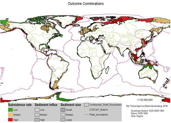
Examples of a coastal typology (top; work of MSc student Maria Karssenberg) used as coneptual model of coastal hydrogeological heterogeneity. Based on this conceptiual model, a large number (100) realizations of coastal heterogeneity (number of aqiuifers/aquitards and conuctivity) is simulated using a Monte Carlo Approach (Middle Figure shows one realization). Each realization is used as input to a SEAWAT model simulating groundwater salinity accross a full glacial cycle (Last high stand untill now: 160,000 years). The average over the 100 realizations (bottom image) provides an estimate of onshore (blue) and offshore (green) fresh groundwater volumes. The light blue line is sea-level across the last glacial cycle (Source: PhD research Daniel Zamrsky). Clicking on the lower figure starts a movie of one simulation.
A palaeohydrogeological reconstruction of the fresh-brackish-salt water distribution in the Nile delta. Input is a paleogeogeographical reconstruction and salinity observations (Top). These ar used as input to a complex 3D variable-density groundwater flow model (2 million cells, 1 km horizontal, 35 layers) using a state-of-the-art model code that allows for parallel computation . The model is run from the latest lowstand (26.5 BP) untitl present day (35 ka). The bottom figure shows the fresh-brackish-saline-hypersaline interfaces (snapshot 13000 BP). Clicking on this figure starts a movie over the enire simulation mperiod. Depending on geological scenario, estimates of fresh groundwater vary between 1500-2300 km3 with offshore groundwater varying between 1-15% respectively (source: van Engelen, J., Verkaik, J., King, J., Nofal, E. R., Bierkens, M. F. P., and Oude Essink, G. H. P., 2019. A three-dimensional palaeo-reconstruction of the groundwater salinity distribution in the Nile Delta Aquifer, Hydrol. Earth Syst. Sci. Discuss., https://doi.org/10.5194/hess-2019-151).
Example publications
- Van Engelen, J., Oude Essink, G.H.P., Kooi, H., Bierkens, M.F.P., 2018. On the origins of hypersaline groundwater in the Nile Delta aquifer. Journal of Hydrology 560, 301-317.
- Zamrsky, D., Oude Essink, G.H.P., Bierkens, M.F.P., 2018. Estimating the thickness of unconsolidated coastal aquifers along the global coastline. Earth System Science Data 10, 1591-1603.
- King, J., Oude Essink, G., Karaolis, M., Siemon, B., Bierkens, M.F.P., 2018. Quantifying Geophysical Inversion Uncertainty Using Airborne Frequency Domain Electromagnetic Data—Applied at the Province of Zeeland, the Netherlands. Water Resources Research 54, 8420-8441.
- Huizer, S., A.P. Luijendijk, M.F.P. Bierkens and G.H.P. Oude Essink, 2019. Global potential for the growth of fresh groundwater resources with large beach nourishments. Scientific Reports 9, 12451.
- Engelen, J., Verkaik, J., King, J., Nofal, E. R., Bierkens, M. F. P., and Oude Essink, G. H. P., 2019. A three-dimensional palaeo-reconstruction of the groundwater salinity distribution in the Nile Delta Aquifer, Hydrol. Earth Syst. Sci. Discuss., https://doi.org/10.5194/hess-2019-151
Global floods and droughts (climate impacts, climate feedbacks and forecasting)
Apart from considering the detrimental effects from human water consumption, the occurrence of floods and droughts due to climate variability and climate change is an important area of research. In this focus area we study a) the effects of climate change on river flow (floods and droughts), b) the relation between land surface conditions evaporation and precipitation recycling, c) seasonal forecasting of river flow and soil moisture. Apart from the global hydrological model PCR-GLOBWB, we also employ statistical analyses and conceptual modelling approaches. Research under this theme is done in close cooperation with Deltares.
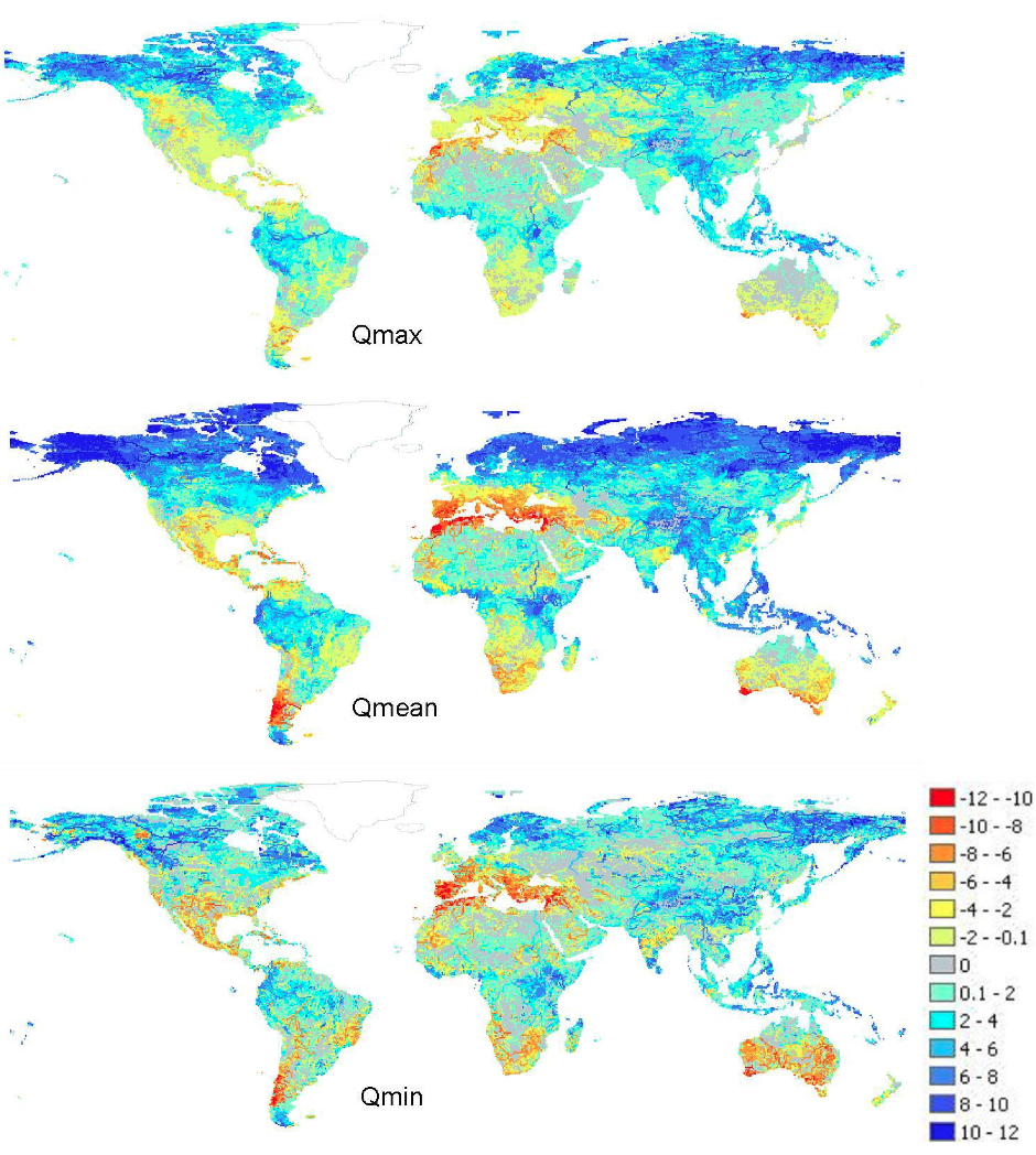
A new way of dealing with multi-GCM uncertainty: maps showing the number of models projecting significant change (compared to GCM-specific year-to-year variation; significance level of 95%) in the same direction as the ensemble mean direction of of change. From top to bottom the figure shows GCM-consistencies for yearly maximum, mean and minimum discharge. Negative values correspond to the number of models showing discharge decrease, positive values correspond to the number of models projecting discharge increase, grey areas correspond to areas with no significant change (Source: Sperna Weiland, F.C., L.P.H. van Beek, J. C.J. Kwadijk, and M.F.P. Bierkens, 2011. Global patterns of change in discharge regimes for 2100. Hydrology and Earth System Science, 16, 1047-1062, 2012)
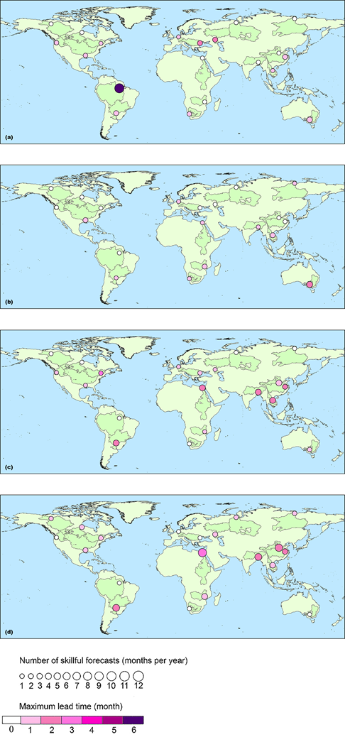
Global overview of the skill for 20 large river basins of ensemble of seasonal streanflow forecasts (monthly time step) obtained by forcing PCR-GLOWB with climate data from 11 ensemble members of the ECMWF S3 seasonal forecasting system. The skill is compared to a reference based on ESP (using an ensemble of 11 randomly sampled years from ERA-40). The added skill is estimated with the Briar skill score (BSS) which compares the ability of the seasonal forecasting system and the ESP forecasting system to correctly predict the occurrence of high flow and low flows (taken als q75 and q25 for each month). A BSS > 0.05 is deemed skillful. The maps show the number of months with skillfull forecasts )irrespective of lead times) and the maximum leadtime for which one finds skill(months). Maps a and b rshow results for high and low flows based on theoretical skill: taking PCR-GLOBWB streamflow forecd with ERA40 as surrogate observations. Maps c and d provide results for high and low flows for actual skill: comparing with GRDC discharge observations (Source: Candogan Yossef, N., van Beek, R., Weerts, A., Winsemius, H., and Bierkens, M. F. P., 2017. Skill of a global forecasting system in seasonal ensemble streamflow prediction, Hydrol. Earth Syst. Sci., 21, 4103-4114).
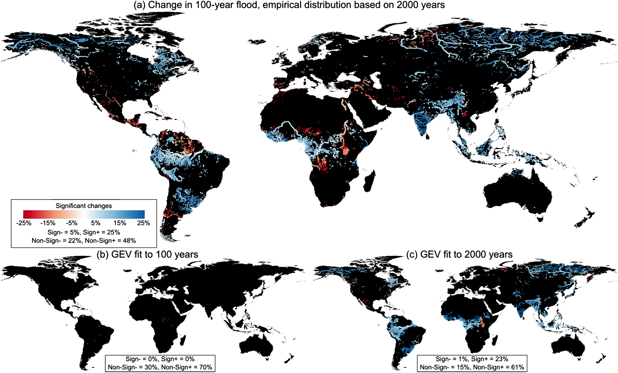
Estimating changes in hydrological extremes using the traditional approach based on observations and fitting extreme value distributions (GEVs) and by direct estimation of exceedance probabilities based on a 2000 years ensemble of climate projections. The Figures show the % of significant change in the 100-year floods for a 2 oC warmer world. In the traditional approach a limited number (say 100 years) of currently yearly maxima is used to fit a GEV distribution. Next, this is repeated for 100 years in a warmer world (from climate model projections, often using a delta-change approach). Due to the large uncertainty of GEV distribution fitted to only 100 years (sampling error), it is difficult to determine any significant change (lower left figure). Simulating 2000 years of discharge based on a very-large ensemble of 2000 years meterological inputs, simullated with the GCM EC-EARTH for current climate and for a 2 degree warmer world, and using these as input for fitting a GEV distribution (lower right figure) picks up much more rivers with significant change in 100-year floods. However, even more signal is picked up (upper large figure) when directly estimating the 100-year floods empirically from the 2000 years of simulated discharges. This is because the strict form of the GEV does not allow the inclusion of compound events with lower probabilities: e.g. large storm systems occurring in two separate braches of the Amazon that result in the confluence of two discharge peaks. (Source: Van der Wiel, K., Wanders, N., Selten, F.M., Bierkens, M.F.P., 2019. Added Value of Large Ensemble Simulations for Assessing Extreme River Discharge in a 2 °C Warmer World. Geophysical Research Letters 46, 2093-2102)
Example publications
- Bierkens, M.F.P. and L.P. van Beek, 2009. Seasonal Predictability of European Discharge: NAO and hydrological response time. Journal of Hydrometeorology 10, 953–968.
- Sperna Weiland, F.C., L.P.H. van Beek, J. C.J. Kwadijk, and M.F.P. Bierkens, 2011. Global patterns of change in discharge regimes for 2100. Hydrology and Earth System Science16, 1047-1062, 2012.
- Candogan Yossef, N., van Beek, R., Weerts, A., Winsemius, H., and Bierkens, M. F. P., 2017. Skill of a global forecasting system in seasonal ensemble streamflow prediction, Hydrol. Earth Syst. Sci., 21, 4103-4114.
- Winsemius, H.C., J.C.J.H. Aerts, L.P.H. van Beek, M.F.P. Bierkens, A. Bouwman, B. Jongman, J. Kwadijk, W. Ligtvoet, P.L. Lucas, D.P. van Vuuren and P.J. Ward, 2016. Global drivers of future river flood risk. Nature Climate Change 6, 381–385.
- Van der Wiel, K., Wanders, N., Selten, F.M., Bierkens, M.F.P., 2019. Added Value of Large Ensemble Simulations for Assessing Extreme River Discharge in a 2 °C Warmer World. Geophysical Research Letters 46, 2093-2102.
Global temperature modelling and the impacts of climate change and water use on energy production and aquatic ecosystems
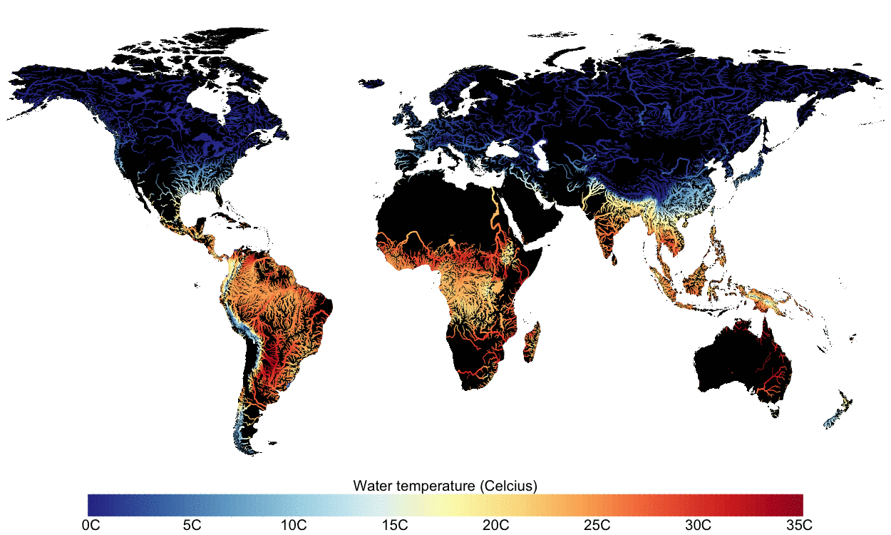
Yearly water temperature climatology based on 30 years of water temperature simulations with DynWat. Dynwat calculates daily surface water temperature by solving the energy balance of flowing water including: the influx of water from precipitation, surface runoff, interflow and groundwater runoff; the surface energy balance (radiation and turbulent fluxes) and lateral transport by advection. It includes a routine to calculate overbank inundation (parameterzied) that increases the area of the surface watre bodies; ice formation, melt and break-up; and a routine to handle lakes and reservoirs where the energy balance is only resolved for the thermally active layer (epilimnion) as long as the temperature profile is stable. This layer is fully mixed over the lake or reservoir depth if the temperature of the epilimnion is low enough to cause instability. In the example shown here, DynWat is forced with runoff and river discharge from PCR-GLOBWB 2, but it can also be forced by the output of any other land surface model. The DynWat code is freely available from Github (https://github.com/wande001/dynWat) (source Wanders,N., van Vliet, M.T.H., Wada,Y.,Bierkens,M.F.P. and van Beek, L.P.H.(Rens), 2019. High-resolution global watertemperature modeling. Water Resources Research 55, 2760–2778).
Both water temperature as well as discharge impact energy production. Hydropower potential depends on discharge and elevation change, while thermo-electric power generation potential depends on discharge and water temperature. In the application below Van Vliet et al. (2016) calculated the change in hydropower and cooling water discharge potential under cliimate change using three global hydrology and temperature models (VIC-RBM, PCR-GLOBWB and WaterGAP2) forced by 5 GCMs.
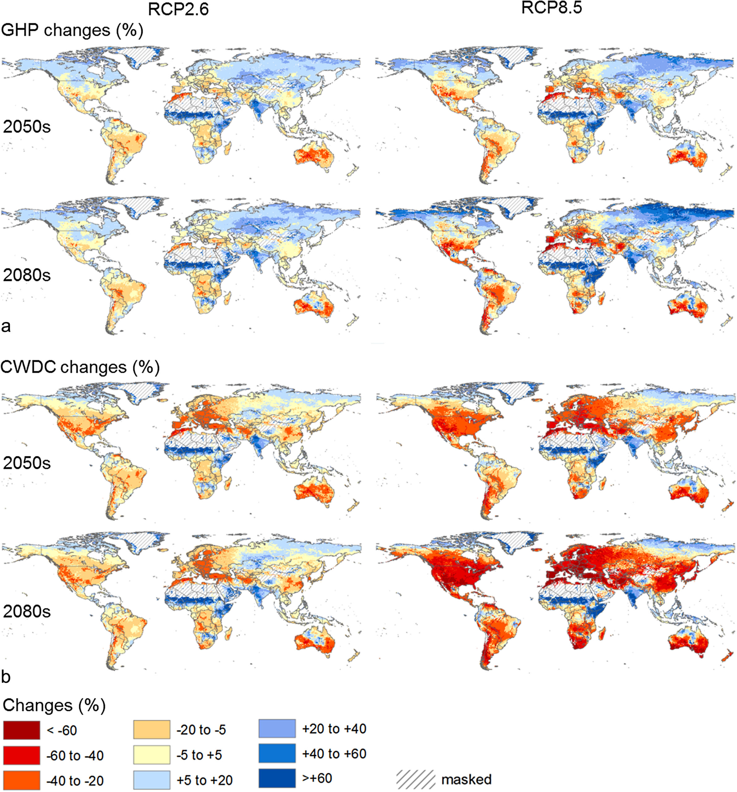
Global spatial patterns of changes in gross hydropower potential (GHP (W); a) and cooling water discharge capacity (CWDC (W); b) based on the ensemble mean of all three GHMs and climate forcing from five GCMs. Changes are presented for the 2050s (2040–2069) and 2080s (2070–2099) for RCP2.6 and RCP8.5 relative to the control period (1971–2000). Regions with mean streamflow less than 1 m3s−1 for the control period are masked because small absolute biases in simulated results can have major impacts on the calculated relative changes in GHP and CWDC (Source: . Van Vliet, M.T.H., van Beek, L.P.H., Eisner, S., Flörke, M., Wada, Y., Bierkens, M.F.P., 2016. Multi-model assessment of global hydropower and cooling water discharge potential under climate change. Global Environmental Change 40, 156-170).
Almost 20% of the catchment areas where groundwater is pumped suffer from a flow of streams and rivers that is too low to sustain their freshwater ecosystems. This number is expected to increase to 50% by 2050. This is the conclusion of our study that appeared in Nature. The study is a collaboration between Utrecht University, the water institute Deltares, the University of Freiburg (Germany) and the University of Victoria (Canada).
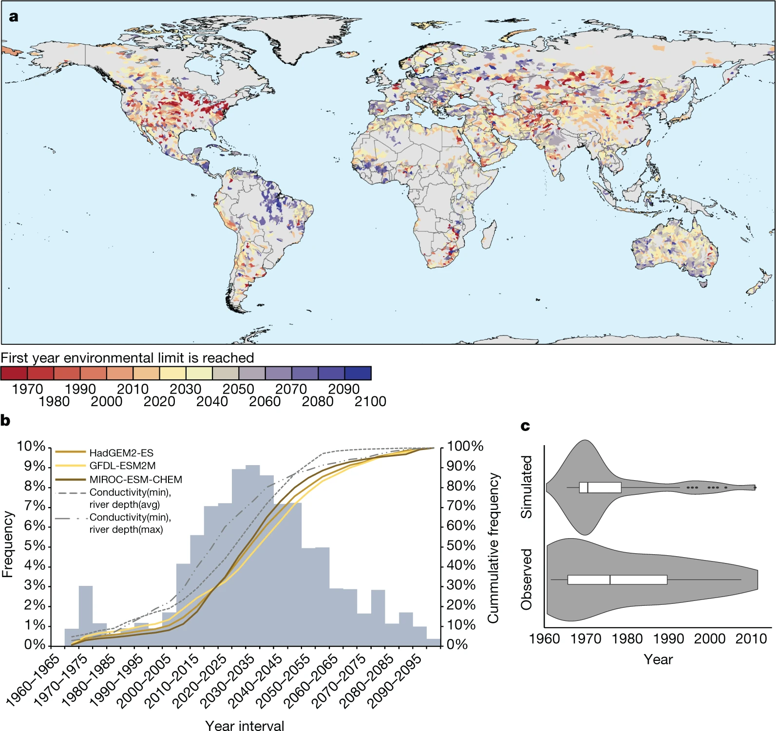
a, The first time at which environmental flow limits have been, or will be, reached, by year, averaged per sub-watershed (using the sub-watershed level of the HydroBASINS dataset23). b, Global distribution of estimated first times at which environmental flow limits have been, or will be, reached. The histogram shows the estimates using the average climate input (HadGEM2-ES). Cumulative frequency is plotted for all three climate inputs used (coloured lines), and for the two runs with different parameter values resulting in the minimum and maximum number of watersheds reaching their environmental flow limit (grey lines, with minimum conductivity values and showing average and maximum river depth). c, Evaluation of this study’s estimations for the first time at which environmental flow limits have been reached (simulated) and ‘observed’ environmental flow limits estimated from streamflow observations for 42 stations in Kansas, USA. The violin plot shows the distribution of the data, the bottom and top of each box represent the 25% and 75% quantiles, and the line inside each box represents the median.
Surface water temperature and discharge impact fresh water systems. In a study in Nature Communications, we worked together with ecologists from Radboud University Nijmegen on projecting the potential impact of global warming on the geographic distribution of 11,5000 freshwater fish. We show that in a 3.2 °C warmer world (no further emission cuts after current governments’ pledges for 2030), 36% of the species have over half of their present-day geographic range exposed to climatic extremes beyond current levels
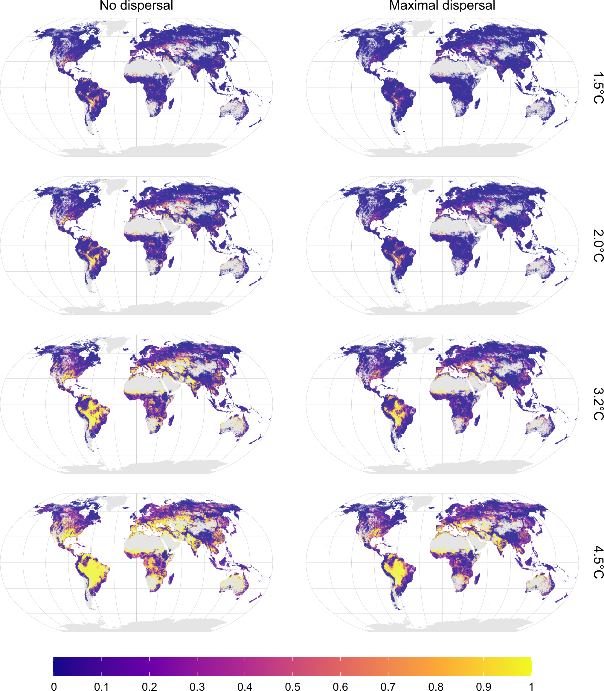
Potentially affected fraction (PAF) of freshwater fish species due to exposure to water flow and temperature extremes beyond current levels, for different global warming levels and two dispersal assumptions. Patterns are based on the median PAF across the GCM–RCP combinations at a five arcminutes resolution (~10 km). Gray denotes no data areas (no species occurring or no data available)
Example publications
- Wada, Y., L.P.H. van Beek, F.C. Sperna Weiland, B.F. Chao, Y.-H. Wu, and M.F.P. Bierkens ,2012., Past and future contribution of global groundwater depletion to sealevel rise, Geophysical Research Letters 39, L09402.
- Wada, Y., L.P.H. van Beek, N. Wanders and M.F.P Bierkens, 2013. Human water consumption intensifies hydrological drought worldwide. Environmental Research Letters 8, 034036.
- Wanders,N., van Vliet, M.T.H., Wada,Y.,Bierkens,M.F.P. and van Beek, L.P.H.(Rens), 2019. High-resolution global watertemperature modeling. Water Resources Research 55, 2760–2778
- Van Vliet, M.T.H., van Beek, L.P.H., Eisner, S., Flörke, M., Wada, Y. and Bierkens, M.F.P., 2016. Multi-model assessment of global hydropower and cooling water discharge potential under climate change. Global Environmental Change 40, 156-170.
- De Graaf, I.E.M., Gleeson, T., (Rens) van Beek, L.P.H., Sutanudjaja E.H, Bierkens, M.F.P. (2019). Environmental flow limits to global groundwater pumping. Nature 574, 90–94.
- Barbarossa, V., Bosmans, J., Wanders, N., King, H., Bierkens, M.F.P., Huijbregts M.A.J and Schipper, A.M. (2021). Threats of global warming to the world’s freshwater fishes. Nat Commun 12, 1701.
Following shortly (pending publiction):
- The impact of terrestrial water storage trends under climate change on regional sea-levels (in preparation)